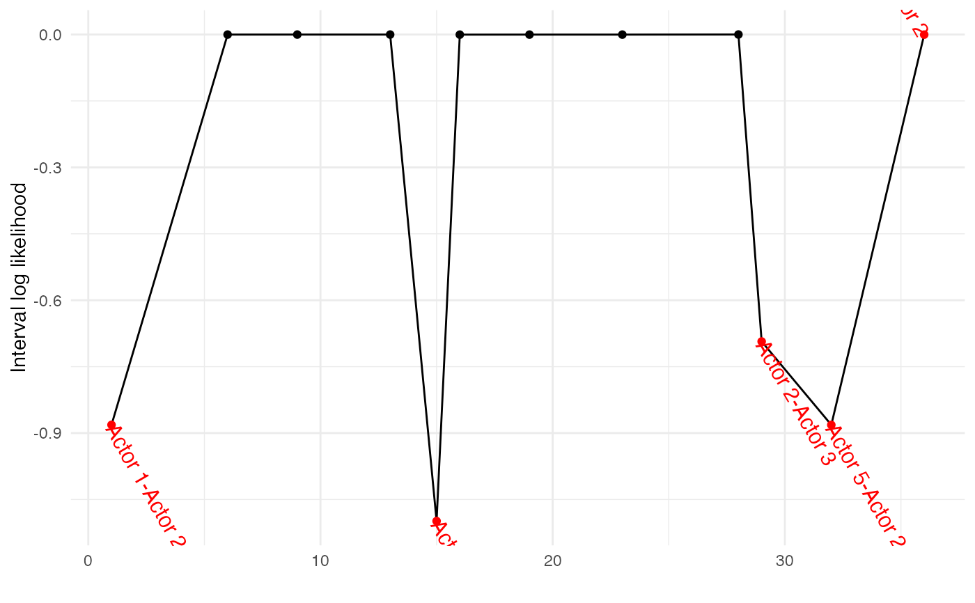
These plotting methods are for diagnosing the adequacy of model specification, such as those used in goldfish. These plots are useful for identifying whether there might be significant outliers affecting the results, whether there is significant time heterogeneity, and which actors' activity the model does not reproduce.
Usage
# S3 method for class 'diagnose_outliers'
plot(x, ...)

# S3 method for class 'outliers.goldfish'
plot(x, ...)

# S3 method for class 'diagnose_changepoints'
plot(x, ...)

# S3 method for class 'changepoints.goldfish'
plot(x, ...)

# S3 method for class 'goldfishOutliers'
plot(x, ...)

# S3 method for class 'goldfishChangepoints'
plot(x, ...)

# S3 method for class 'goldfishMargins'
plot(x, ..., top = 25)

# S3 method for class 'goldfishGOF'
plot(x, ..., level = 0.95, page = NULL, nrow = 2, ncol = 2)

# S3 method for class 'goldfishTimeTest'
plot(x, ..., page = NULL, nrow = 2, ncol = 2)

# S3 method for class 'goldfishOnset'
plot(
  x,
  ...,
  view = c("both", "path", "accrual"),
  tolerance_band = TRUE,
  page = NULL,
  nrow = 2,
  ncol = 2
)
Arguments
- x
An object of class
goldfishOutliers,goldfishChangepoints,goldfishMargins,goldfishGOF,goldfishTimeTestorgoldfishOnset, as returned bydiagnose_outliers(),diagnose_changepoints(),margin_table(),test_gof(),test_time()anddiagnose_onset()in goldfish.- ...
Additional plotting parameters, currently unused.
- top
The number of actors to draw, those furthest from the reference.
- level
The confidence level of the reference bands, defaulting to 0.95. The band is the two-sided Kolmogorov quantile of the supremum of a Brownian bridge, which is the reference the event-clock p-value uses.
- page
Which page to draw, for the per-term figures.
NULL(the default) draws every panel in one figure, exactly as before. A number draws that page alone; a number past the last is an error naming the count. Usecount_pages()to learn the count without rendering, so a loop can write every page with nobody at a screen.- nrow, ncol
Panels per page when
pageis given.- view
Which panels to draw:
"both"(default), or"path"or"accrual"alone, which is the escape hatch when a model has too many coefficients for a composed figure to stay readable.- tolerance_band
Whether to draw each coefficient's stabilization band, the
+/- tolerance * std_errorcorridor the path had to re-enter.
Details
plot.diagnose_outliers(), plot.outliers.goldfish(),
plot.diagnose_changepoints() and plot.changepoints.goldfish() are
aliases for plot.goldfishOutliers() and plot.goldfishChangepoints(),
kept so that an object carrying one of the older class names plots as
before. Each reads the columns the current methods read. They will be
removed.
goldfish emits these objects plot-ready. Each is a tibble carrying the diagnostic metadata contract — which function produced it, which model and sub-model it came from, and the arguments that shape how it is read — so these methods take their series, their labels and their reference lines from the object rather than inferring them from the columns that happen to be present.
The .series column is the series the diagnostic actually analysed: the
per-interval log-likelihood by default, and the selected term's own
series when the diagnostic was called with effect =. It is NA on the
intervals that took no part, which on a rate or REM fit are the
right-censored ones.
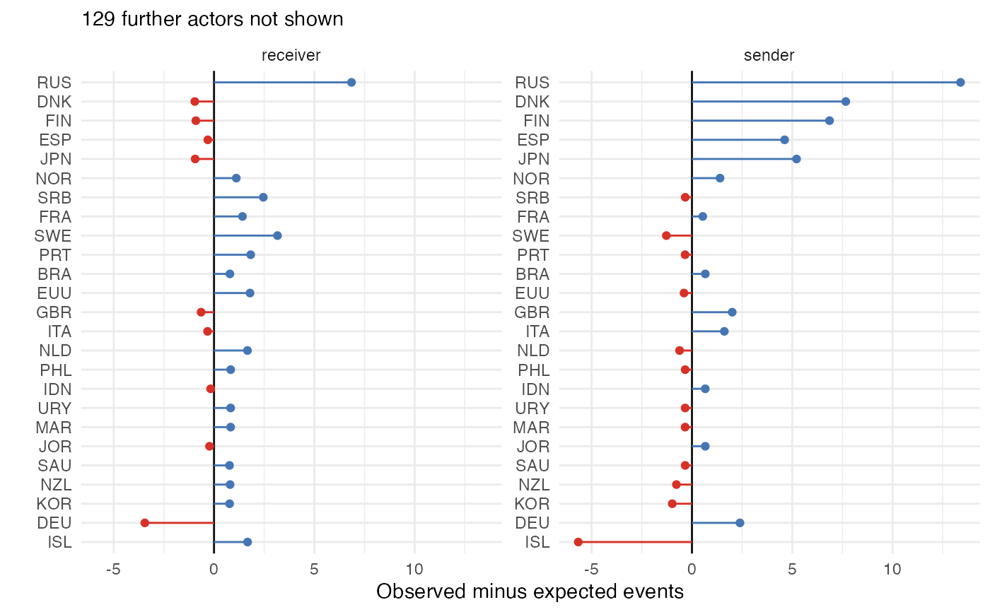
plot.goldfishMargins() shows each actor's observed activity against what
the model expected of them. Which comparison it draws follows the scales
the fit's model class defines, which the object records: where a
compensator is defined (the exact-time sub-models) the difference
observed - expected_count is the per-actor martingale residual, read
against zero; on the multinomial sub-models, which have no exposure-time
term and so no compensator, the ratio observed / expected_probability
is a calibration ratio, read against one.
These are descriptives rather than per-actor tests: the differences are plug-in quantities and are negatively correlated across actors. Read the plot as a map screening for unmodelled actor heterogeneity.
A node set large enough to make one row per actor unreadable is the
ordinary case, so only the top actors furthest from the reference are
drawn, and the subtitle says how many were left out. Actors are ranked by
their largest deviation over the roles they appear in, so an actor kept
for one margin keeps the other beside it. Pass top = Inf for all of
them.
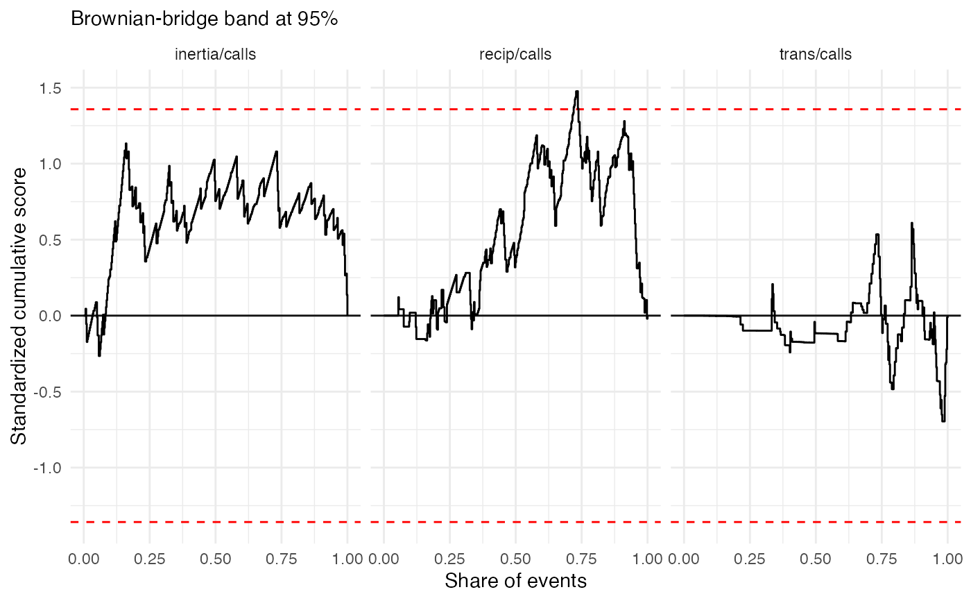
plot.goldfishGOF() draws each effect's standardized cumulative score
process against the Brownian-bridge bands its p-value was read from. At
the maximum the per-event scores sum to zero, so every path starts and
ends at zero; under a correctly specified model it is a bridge, and a path
that wanders outside the bands is an effect whose contribution is
concentrated somewhere in the sequence.
The x axis is the object's own process-time axis, taken from its u
column and labelled by the clock it records. This is not a
presentational detail: the bands are valid on whichever clock produced the
process, and re-deriving an event-index axis here would draw the path on
one clock and the reference on another. On the information clock the
spacing of the steps is itself the diagnostic — a path that crosses most
of the axis in a few steps is an effect whose information arrives late.
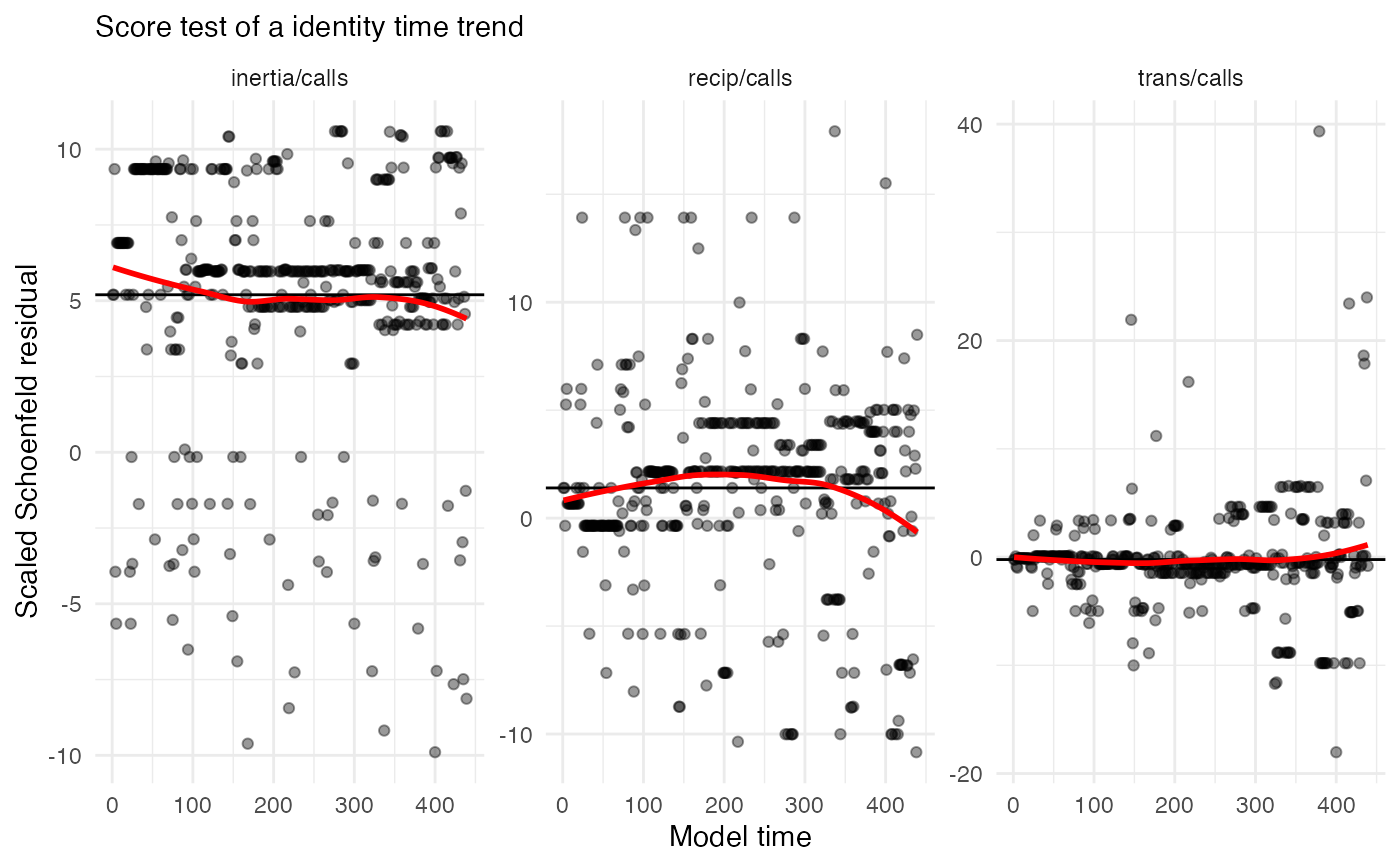
plot.goldfishTimeTest() draws the scaled Schoenfeld residuals of each
tested effect against time, with a smooth and the fitted estimate as the
reference. A residual scatter is centred on the coefficient the model
estimated; a smooth that drifts away from that line over the sequence is
the coefficient failing to be constant, which is what the test's p-value
states formally.
Under method = "periods" the intervals are coloured by their period, so
the regimes the test compared are visible against the same scatter.
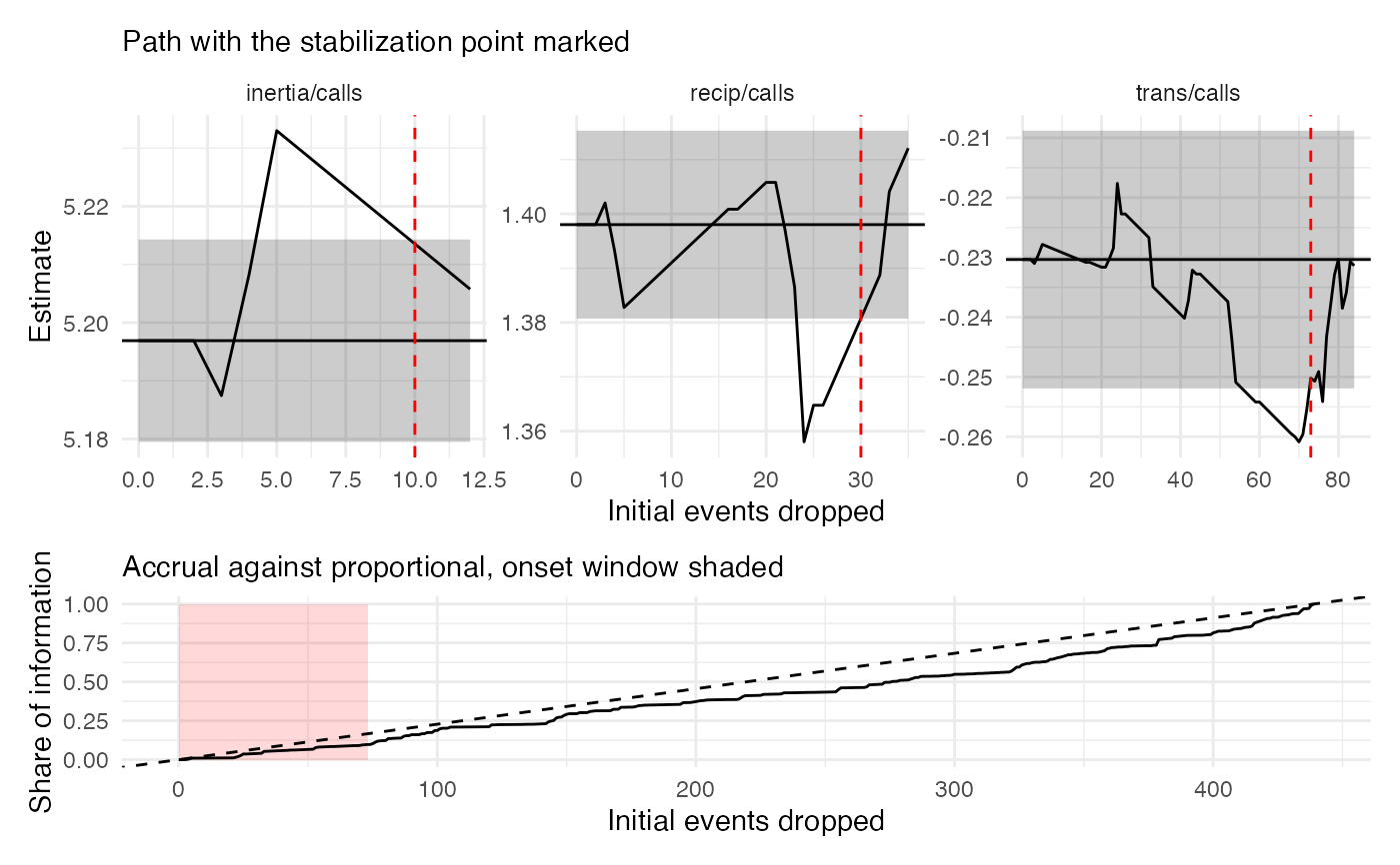
plot.goldfishOnset() composes two panels: each coefficient's
leave-the-first-m-events-out path, and the share of the model's
information those events delivered.
Both panels are windowed on the excursion rather than the sequence, because the full range is mostly bridge tail — the path returns to the estimate by construction, so drawing all of it squashes the part being read into a few percent of the axis. Each coefficient gets its own window and its own x scale, since coefficients settle at very different points and a window shared across facets re-creates the squashing it exists to prevent. A coefficient whose path never left its band takes the full range, there being no excursion to window on.
The accrual panel is drawn full-range with the onset window shaded, and
carries the proportional diagonal y = x / n. Without the diagonal a
monotone curve from 0 to 1 says nothing: the signal is the departure
from proportional, which is what makes an opening segment that carries
little information visible.
Coefficients held fixed through offset() are not drawn. Their path is a
flat line at the imposed value by construction.